01.1 Deep learning and long-term investing · Pre-registered
Deep Portfolio Constructor
In plain English
Can an AI grow a dollar more than simply buying the whole US stock market and holding it?
- The question Put $1 into the US stock market in 1960 and leave it alone. Could an AI that adjusts the mix every month end up with more?
- What it does Every month it looks at 30 parts of the economy, from food to health to banks, and decides how much to hold in each. It never bets against a company and never borrows.
- How it learned It practised on decades of history and was judged on one thing only: how much money it would end with after paying for every trade. It was always tested on years it had never seen.
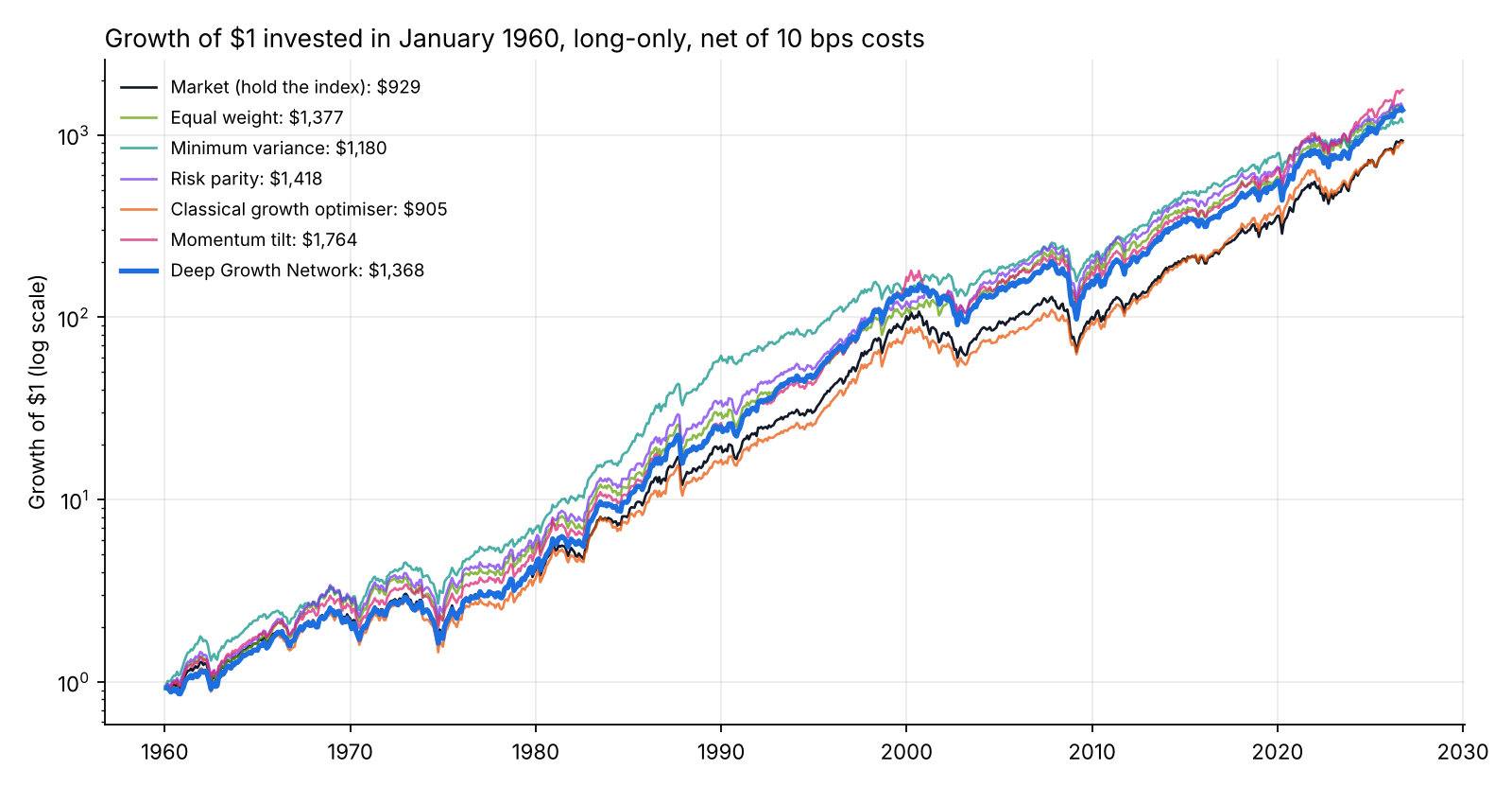
- The honest result $1 became $1,368, against $929 for simply holding the market. I wrote the pass mark down before running the test, and this gap is too small to rule out luck. The site says so.
A neural network that builds a long-only portfolio for long-term wealth, trained on the growth of wealth after every trading cost.
What it provesTrained only on the growth of wealth, the network turned $1 in 1960 into $1,368, against $929 for the market: +0.58% a year, a gap the pre-registered test cannot tell from luck (t = 1.40).
A transformer that allocates across Kenneth French's 30 US industries, trained in PyTorch on the growth of wealth itself through a differentiable simulator of buying, holding and paying to trade, walk-forward from 1960 and tested out of sample against the market and five classical long-only strategies.
Stack Python, PyTorch, pandas, NumPy, cvxpy, statsmodels, pytest
Objective
Grow wealth over decades: buy, hold, and trade only when it pays.
A long-term investor keeps the compound growth of their wealth, and that is not the average return. Volatility drags compounding down (growth is roughly the average return minus half the variance), and the cost of every trade compounds too. So this network is not trained to forecast returns. It is trained on the quantity the investor keeps: the growth of wealth after costs, the .
The rules are a patient investor's: long-only, fully invested, no leverage, no shorting, no jumping into cash. The universe is Kenneth French's 30 US industry portfolios, which at every date hold every listed firm in the industry, including the ones that later failed, so there is no . The question, fixed in advance: can a neural network beat simply holding the market, out of sample from 1960?
Try it
Why the network is trained on growth, not on average return.
Two made-up assets: a steady market and a riskier industry with a higher average return. Slide toward the risky one. The average return rises all the way; the wealth it compounds into peaks, then falls, because volatility drains growth. The network's loss is the second curve.
- Average return
- 13.0%
- Volatility
- 30.0%
- Growth per year
- 8.5%
- $1 after 66 years
- $273
100% risky has the higher average return (13.0%) but volatility drags growth down to 8.5%: $273 after 66 years, against $475 at 46%.
The deep stack
A transformer that tilts the index, learns when not to trade, and learns from the wealth it ends up with.
- Inputs known at each month-end. For every industry, 13 features: returns over 1, 3, 12 (skipping the last month), 36 and 60 months, volatility over 1 and 5 years, downside risk, drawdown, beta and correlation with the market, book-to-market and its weight in the index, plus where the current holding sits against the market. For the market as a whole, 7 more: its trend over 1 and 5 years, volatility, drawdown, valuation, the spread between industries and the T-bill rate.
- Attention across industries. Each industry is a token, with one more for the market; two blocks let every industry weigh every other before the network decides. 20,066 parameters.
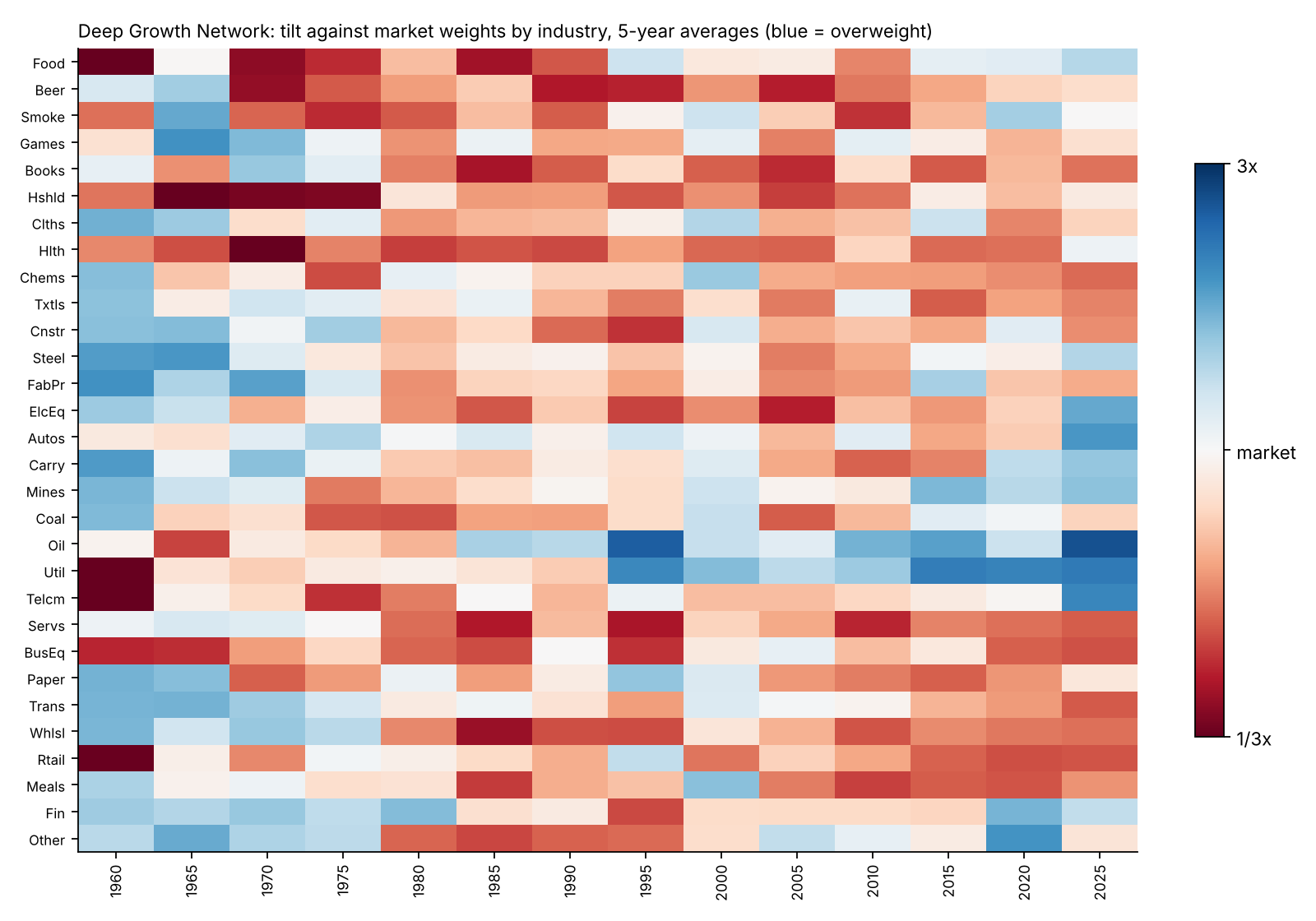
- Long-only by construction. The network tilts the market's weights: each industry's weight is multiplied by a factor between a third and three, then the portfolio is rescaled to 100%. Always fully invested, never short, never levered. The tilt starts at zero, so an untrained network holds exactly the market and has to earn every deviation from it.
- A learned trade fraction. A second head reads the market token and decides how much of the gap between today's holdings and the target to trade this month: none of it is buy and hold, all of it a full rebalance. How much to trade is learned, not set by hand.
- Trained on the outcome. A plays the investing rules forward: holdings drift with prices, every trade costs 10 bps, and the loss is minus the log growth of wealth over five-year episodes. Gradients flow back through 60 months of compounding, so a trade today is judged by the years after it.
- Walk-forward, pre-registered. The network is refit every five years on past data only (), with the last ten years of each window held out to decide when to stop training. Five seeds; the deployed policy averages them. The protocol, the comparisons and the decision rule were in git before the network was run out of sample.
How it learned
70 networks, each trained on the past only and stopped by years it never trained on.
The deployed policy is not one network. At each refit, every five years from 1959, five seeds are trained on data before the last ten years, those ten years decide when to stop, and the five targets are averaged. Pick a refit to watch its five seeds learn.
At the first refit every seed starts as the market, because the tilt head is zero at birth, and the median seed found +1.6% a year of extra growth on the validation decade. After that each seed starts from its own network of five years earlier, and in 22 of 65 of those refits early stopping found nothing better and kept it: the network is allowed not to change its mind. Training all 70 took 1.3 hours of wall-clock time.
Training step. Up is faster growth of wealth on the validation years, % a year, against where training started.
- Seeds that improved
- 5 of 5
- Median gain kept
- +1.6%
- Validation years
- 1950–1959
- Then used for
- 1960–1964
Trained on data before 1950, stopped on 1950–1959, then trusted with 1960–1964. Every seed began as the market. All 5 found weights that grew wealth faster on the validation years.
Results
Out of sample from 1960, the network's edge over simply holding the market is too small to tell from luck.
$1 invested in January 1960 became $1,368 with the network and $929 in the market: 11.43% a year against 10.78%. The yearly difference in log growth is +0.58%, with a Newey-West of 1.40 and a 95% block-bootstrap interval of −0.07% to +1.50%: no detectable difference. It traded 155% of the portfolio a year, an average holding period of 0.6 years, and its weights differed from the index's by 32% on average ().
It did not learn to sit still: its trade fraction started training at 25% and settled at a median of 81%, chasing a target that moved every month. It leaned toward value, with a value-factor loading of 0.17 against the market's 0.01; after adjusting for market, size and value, its alpha is +0.15% a year ( = 0.38).
The strongest classical rival is a simple momentum tilt, +0.96% a year above the market. Against it the network's difference is −0.38% (t = −0.69): no detectable difference. Against the classical growth optimiser, which chases the same goal with estimated returns and risks: +0.62% (t = 1.05): no detectable difference.
Pick a strategy to see its path and what it did differently. The full table is under the chart.
$1 invested in January 1960 · pick a strategy
Growth of $1 since 1960, log scale · Deep Growth Network
- $1 became
- $1,368
- Per year ()
- 11.43%
- Worst
- −52%
- Traded per year
- 155%
Against the market: +0.58% a year of growth, = 1.40: no detectable difference.
Market. Buy every industry at its market weight and hold it: the index fund most professional managers fail to beat. $1 in 1960 became $929, 10.78% a year, trading only 4% of the portfolio a year as the index itself changes.
Equal weight. Put 1/30 in every industry each January and sit: a bet on the smaller industries. +0.59% a year against the market ( = 0.87): no detectable difference.
Minimum variance. The lowest-risk long-only mix and the smoothest ride (worst fall −41% against the market's −50%), but it lags whenever the largest industries lead. +0.36% a year against the market ( = 0.33): no detectable difference.
Risk parity. Equal risk from every industry, rebalanced each January. +0.63% a year against the market ( = 0.94): no detectable difference.
Classical growth optimiser. The textbook version of the network's own goal: maximise from estimated returns and risks, inside the same bounds. $1 became $905, −0.04% a year against the market ( = −0.09): no detectable difference.
Momentum tilt. Overweight the industries that rose most over the past year. +0.96% a year against the market ( = 2.93): better. The price: it trades 110% of the portfolio a year.
Deep Growth Network. A trained on the growth of wealth itself, through a that charges for every trade. $1 became $1,368: +0.58% a year against the market ( = 1.40), too small to tell from luck by the pre-registered test. It trades 155% of the portfolio a year and moves a median 81% of the way from its holdings to its target each month.
Dashed amber: the S&P 500 with dividends reinvested, $831. Shaded: months when the market was 20% or more below its previous peak. Long-only, fully invested, every trade costs 10 bps, out of sample from January 1960 to 2026. Kenneth French's 30 US industry portfolios, which include the firms that later failed. Read from the project's committed results (2f4613a).
A long-term investor does not get to pick 1960. Slide the start year to see what $1 became from any January to today.
- $1 became, network
- $1,368
- $1 became, market
- $929
- Per year, network
- 11.43%
- Per year, market
- 10.78%
Invested in January 1960 and left to the rules until September 2026: the network ended ahead, 11.43% a year for the network against 10.78% for the market.
Against the S&P 500 and the NASDAQ
Added after the pre-registered test, as context: the test's benchmark stays the whole US market. With dividends reinvested, $1 in the S&P 500 at the end of 1959 became $831 (10.60% a year). The network's difference from it is +0.75% a year ( = 1.56): no detectable difference.
The NASDAQ Composite starts in February 1971, and its free history has no dividends, so it is understated. From then, $1 became $265 in the NASDAQ, $360 in the S&P 500, $388 in the whole market and $586 with the network: +1.43% a year against the NASDAQ (t = 0.84): no detectable difference.
Sources: Yahoo Finance's S&P 500 total-return index (from 1988), S&P 500 prices and the NASDAQ Composite, with S&P 500 dividends before 1988 from Robert Shiller's monthly data. Where both exist, the joined series tracks the official total-return index with a correlation of 0.9999.
Inside the portfolio
What the network actually held: drag through 66 years.
Each pair is one industry: the outline is the market's weight, the bar the network's. Press play to watch its holdings through the oil shocks of the 1970s, the technology boom, 2008 and 2020, or point at an industry to read its weights.
Month2026-09
- Biggest overweight
- –
- Biggest underweight
- –
- Differs from the index
- –
- Traded this month
- –
Point at an industry to see its weight.
How often to trade
The same network, rebalanced every day, month, quarter or year. Once a month, the schedule it was trained for, grew the most.
Nothing is retrained. Each schedule runs the trained network on the same 66 years and pays the same 10 bps per trade; only how often it trades changes. This was added after the pre-registered test, which judged the monthly schedule only.
- Every month, as tested: at each month-end it reads the latest data, sets a target and moves most of the way there.
- Every quarter or every year: the network is asked only at the end of each quarter, or only each December. In between, prices move the holdings and nothing is traded.
- Every day: the network still decides at each month-end, because its inputs are monthly. Then at every daily close the portfolio is traded back to the mix it chose, using Kenneth French's daily industry returns. As a check, trading only at month-ends on the daily data gives $1,388, against $1,368 from the monthly engine.
Trading every day only keeps the portfolio at the month's chosen mix, and it costs more: 0.44% a year against 0.31%. Trading less often costs less (0.05% a year once a year) but lets the tilts go stale: once a year it grew −0.04% a year against the market. That suggests what the network knows about each industry fades within months.
- $1 became
- $1,368
- Before costs
- $1,685
- Traded per year
- 155%
- Cost per year
- 0.31%
Against the market: +0.58% a year of growth, = 1.40: no detectable difference.
As tested: at each month-end it reads the latest data, sets a target and moves most of the way there.
Decade by decade
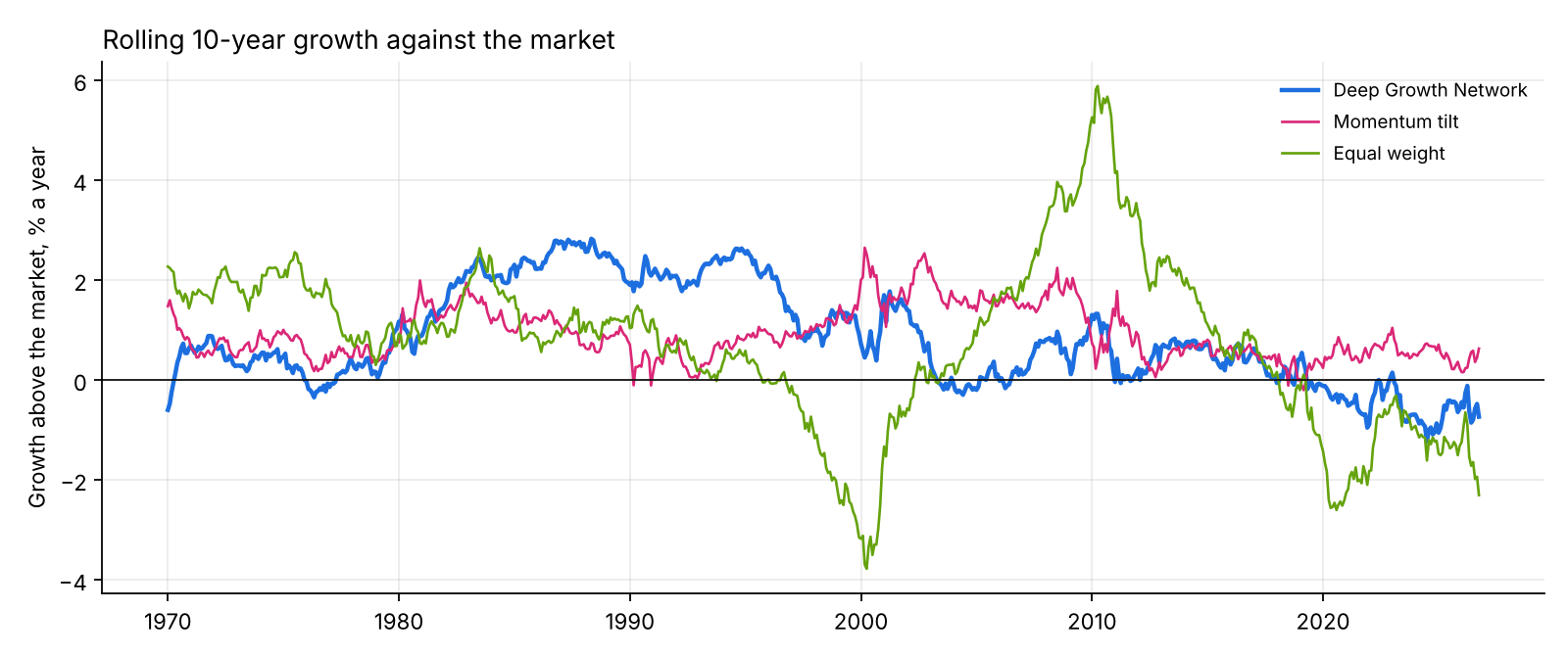
Long-term wealth is made over decades, so the comparison is too.
In 79% of the rolling ten-year windows since 1960 the network grew faster than the market; the momentum tilt did in 99%.
What each part adds
Switch off one idea at a time.
Each ablation was fixed in the protocol and trained with two seeds, 42 and 43, so it is compared with the full network averaged over the same two seeds, which turned $1 into $1,026.
- No learned trade fraction (it trades all the way to its target every month): $1,775, trading 252% a year; +0.82% a year against the full network ( = 1.83): no detectable difference.
- No attention (each industry is judged on its own features and the market's, never against its peers): $701, trading 91% a year; −0.57% a year against the full network ( = −1.57): no detectable difference.
- No market anchor (it allocates from scratch with no bounds; untrained, it holds equal weights): $387, trading 354% a year; −1.46% a year against the full network ( = −0.55): no detectable difference.
Robustness
- Seeds. Each seed's network on its own turned $1 into $1,794, $574, $1,731, $1,091, $1,066: 4 of 5 ended above the market. The deployed policy averages the five.
- Costs. The same decisions re-priced: +0.88% a year against the market with free trading, +0.13% at 25 bps a trade and −0.63% at 50 bps.
- Risk. Volatility 15.1% a year against the market's 15.3%; worst calendar year −39% against −36%; market 0.98.
- Factor-adjusted. Fama-French three-factor alpha +0.15% a year (t = 0.38): what its tilts earned beyond exposure to the market, small firms and value.
Limits
Industries, not funds: an investor in 1960 could not buy these 30 portfolios cheaply, and sector funds came decades later. Costs are a flat 10 bps a trade, with no taxes or market impact; a taxable investor also pays tax on realised gains, which favours trading even less.
The features carry hindsight. Momentum, value and low volatility were documented by finance research long after 1960, so the network was handed inputs an investor then would not have known to look at. The pre-registration fixes the test, not the feature list.
One country, one century: the US market from 1960 was among the best in the world, and five seeds of one network on one history is a small sample. Several strategies were compared; the pre-registered primary test is the one to read.
Checks
106 automated tests, including: the PyTorch simulator reproduces the NumPy backtest engine month by month; an untrained network holds exactly the market; every portfolio is long-only and fully invested; no training label is dated inside the validation window; and the features at any date are the same whether or not later data exists.
The market portfolio rebuilt from the 30 industries tracks French's own market return with a correlation of 0.9998. As calibration, a deliberately cheating policy that sees next month's returns, inside the same bounds and costs, turns $1 into $729 million: the simulator pays for real foresight, so an honest result should look nothing like that.
The protocol is docs/wealth_protocol.md, committed before the out-of-sample run.
Figures on this page are read from data/projects.json, copied from the project's committed reports/site_wealth.json.